
STAP—space-time adaptive processing—is not a single component or a fixed algorithm. In GNSS anti-jamming, it is a processing architecture that combines an antenna array with time-delayed signal taps and adapts the weights jointly across space and time. The goal is practical: suppress interference while preserving the weak GNSS signals that the receiver needs for acquisition, tracking, and timing.
A useful working definition is this: STAP in GNSS anti-jamming is a joint angle-and-frequency filtering method that uses multiple antenna elements and tapped delay lines to place nulls against jammers, including wideband, pulsed, swept, or multiple interferers.
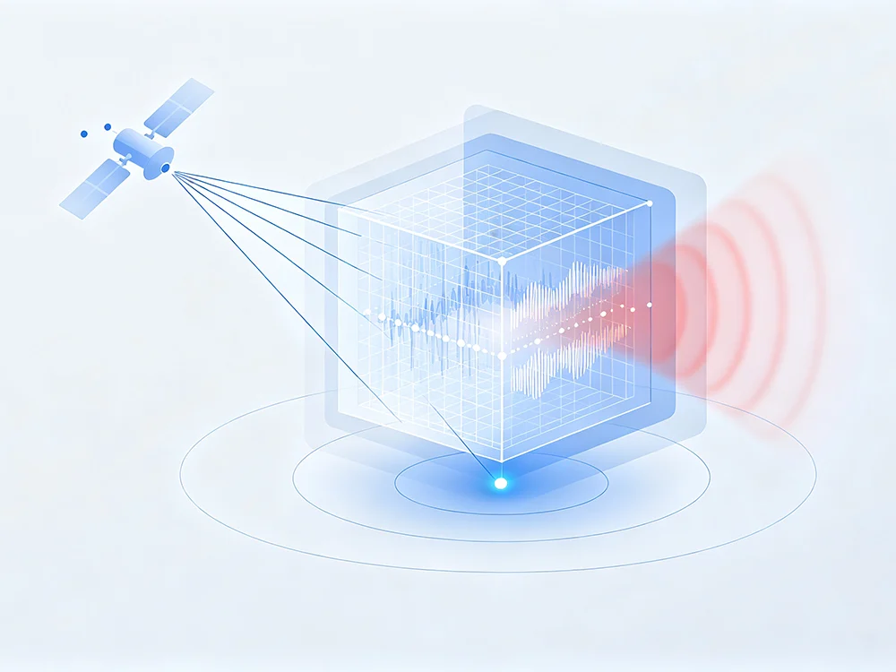
Where STAP sits in a GNSS anti-jamming chain
In a typical receiver architecture, STAP follows the per-element RF/digital front end and precedes acquisition and tracking. Each antenna element has its own digitized signal path. Those streams are combined with delayed versions of themselves, and an adaptive processor calculates complex weights. The weighted output is then passed to the GNSS receiver baseband.
This placement matters. STAP must operate before the receiver loses lock, but it must also avoid distorting the satellite signals it is meant to protect. That is why constrained adaptation and array calibration are central design topics, not optional refinements.
How STAP works without drowning the GNSS signal
A simplified space-time snapshot contains samples from M antenna elements and N time taps. The processor applies a weight vector to that snapshot and minimizes output power subject to one or more constraints. In GNSS, the constraints usually preserve gain in the satellite steering directions so that the anti-jamming filter does not simply null the signals of interest.
The adaptation engine estimates a space-time covariance matrix from received snapshots and updates weights using methods such as sample matrix inversion, recursive least squares, or least mean squares. Diagonal loading is often used to improve robustness when sample support is limited or the covariance estimate is noisy.
The table below shows why STAP is different from spatial-only or time-only filtering.
| Criterion | Spatial-only beamforming | Time-only filtering | STAP |
|---|---|---|---|
| Degrees of freedom | Number of antenna elements | Number of time taps | Elements × taps |
| Main strength | Separates interference by direction | Separates interference by frequency/time signature | Joint angle-frequency discrimination |
| Wideband or pulsed jammers | Limited | Better for some waveforms | Strong when DoF and bandwidth fit |
| Moving interferers | Needs fast adaptation | No angle discrimination | Better tracking with adaptive updates |
| GNSS distortion risk | High near nulls | Moderate | Moderate to high unless constrained |
| Compute and SWaP | Low to moderate | Low | High |
STAP is most valuable when interference is wideband, dynamic, or arrives from multiple directions. It is less attractive when size, weight, power, and cost are tightly constrained and a simpler spatial filter can meet the threat model.
What STAP buys—and what it costs
The benefits are straightforward: deeper nulls against complex interference, better handling of multiple jammers, and the ability to discriminate interference that shares a direction with GNSS signals but differs in time-frequency behavior. The costs are equally real: more channels, more computation, more calibration effort, and more opportunities for signal distortion.
A practical design review should track several metrics together, not just null depth.
| Design factor | Why it matters | Practical watch point |
|---|---|---|
| Array size (M) | More spatial degrees of freedom | Aperture and platform constraints |
| Time taps (N) | More temporal degrees of freedom | Latency and compute grow with M × N |
| Constraints | Protect GNSS steering vectors | Poor constraints can bias code and carrier |
| Adaptation algorithm | Sets convergence and sample support | Fast changes may outrun the estimator |
| Diagonal loading | Stabilizes covariance inversion | Too much loading weakens nulls |
| Calibration | Preserves amplitude and phase response | Drift over temperature and aging |
| Output monitoring | Confirms receiver performance | Watch C/N0, not only output power |
A common rule of thumb is that the available degrees of freedom must exceed the number of interferers plus the constraints used to protect GNSS signals. In practice, margin is needed for calibration errors, multipath, and nonstationary interference.
Integration considerations
STAP does not replace good antenna placement, interference detection, or receiver-level robustness. It works best as part of a layered anti-jamming design. System engineers should define the threat model first, then size the array and taps, then select the adaptation method and constraints. Testing should include live-sky GNSS, simulated jammers, dynamic scenarios, and receiver-level metrics such as acquisition time, tracking jitter, and timing stability.
For a receiver-level view of hardware and interface decisions, see How to Integrate an Anti-Jamming Module into a GNSS Receiver. That guide complements the STAP discussion by focusing on power, interfaces, calibration, and test workflow.
Bottom line
STAP is a powerful but demanding GNSS anti-jamming technique. It earns its place when interference is too complex for spatial-only filtering and when the platform can support the additional degrees of freedom, computation, and calibration. The key is not simply adding more taps or elements; it is constraining the processor so that it suppresses interference without degrading the GNSS signals the receiver depends on.